Practice 2: 3Dimensional reconstruction

In this practical, a 3-D reconstruction was required from the images obtained by two cameras, placed side by side, of a scene. The process followed to carry out this reconstruction is as follows:

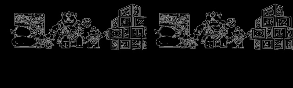
1) Choose which points of interest we want to convert to 3D. In this case, we have selected the edges of the image as points of interest, using the Canny algorithm to calculate these edges. We can see this procedure in the image below

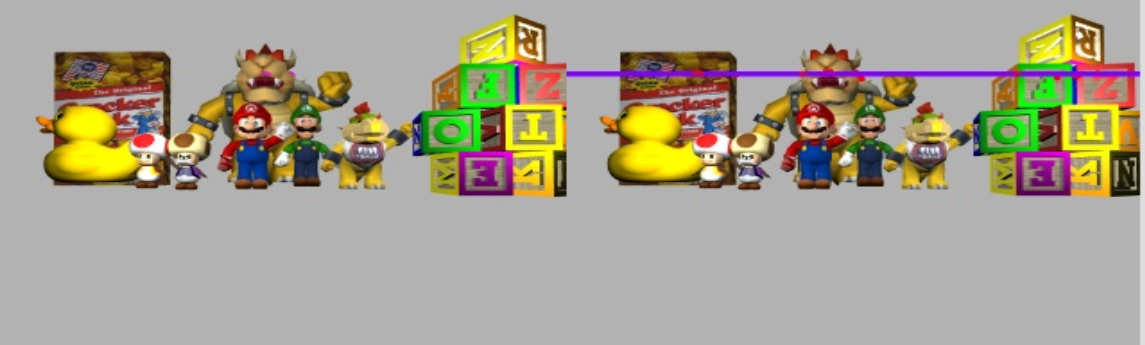
2) Find the homologous pixel in the right image. To do this, we must apply two constraints: the epipolar constraint and the attentive constraint. The epipolar constraint involves starting from a pixel in the left image that we want to convert to 3D, launching a back-projection ray that passes through the pixel in space and through the optical center of the camera. At some point along this ray, we will find the point in 3 dimensions. By projecting this ray onto the other camera, we will have found the epipolar line, and somewhere on this line will be the homologous pixel of the one in the left image that we had selected. To account for precision limitations, we select an epipolar stripe with a margin of 3 pixels above and below the line. Again, we can see the epipolar projected on the right image in the following image.

The attentive constraint requires that if a pixel was an edge in the left image, it will also be an edge in the right image.

In addition, a third constraint has been introduced in this work to speed up the process even further. This constraint is based on the fact that the homologous pixel of the left image in the right image must be located within a square region of 61x61 px² centered around that pixel.

3) Once we have found the homologous pixel, we launch a back-projection ray passing through the optical center of the right camera and look for the intersection with the other ray. Due to numerical accuracy problems, these rays will rarely intersect, so we must find the point of minimum distance between the two lines.

To find the minimum distance between two lines in 3D space, we need to find the points on each line that are closest to the other line. We can do this by minimizing the distance between the two lines, which is equivalent to finding the minimum of the distance function \(D(t_1, t_2) =\)||\((a_1 + t_1b_1) - (a_2 + t_2b_2)\)||

To minimize \(D(t_1, t_2)\), we can take the partial derivatives of D with respect to \(t_1\) and \(t_2\), and set them equal to zero. This gives us two equations in two unknowns, which we can solve for \(t_1\) and \(t_2\).

To set up these equations, we first need to expand \(D(t_1, t_2)\) using the dot product and vector arithmetic:

\[D(t_1, t_2) = ||(a_1 + t_1 b_1) - (a_2 + t_2 b_2)||=\] \[= ||a_1 - a_2 + t_1b_1 - t_2b_2||=\] \[= ||(a_1 - a_2) + t_1b_1 - t_2b_2||=\] \[= \sqrt{((a_1 - a_2 + t_1b_1 - t_2b_2)\cdot(a_1 - a_2 + t_1b_1 - t_2b_2))}=\] \[= \sqrt{((a_1 - a_2)\cdot(a_1 - a_2) + 2\cdot(a_1 - a_2)\cdot(t_1b_1 - t_2b_2) + (t_1b_1 - t_2b_2)\cdot(t_1b_1 - t_2b_2))}=\] \[= \sqrt{((a_1 - a_2)\cdot(a_1 - a_2) + 2t_1b_1\cdot(a_1 - a_2) - 2t_2b_2\cdot(a_1 - a_2) + t_1^2b_1\cdot b_1 - 2t_1t_2b_1\cdot b_2 + t_2^2\cdot b_2\cdot b_2)}\]

We can now take the partial derivative of D with respect to \(t_1\) and set it equal to zero:

\[\dfrac{dD}{dt_1} = (b_1\cdot b_1)\cdot t_1 - (b_1\cdot b_2)\cdot t_2 + b_1\cdot(a_1 - a_2) = 0\]

We can also take the partial derivative of D with respect to t_2 and set it equal to zero:

\[\dfrac{dD}{dt_2} = -(b_1\cdot b_2)\cdot t_1 + (b_2\cdot b_2)\cdot t_2 - b_2\cdot(a_1 - a_2) = 0\]

These two equations can be written in matrix form as:

\[\left[A\right]\left[t\right] = \left[b\right]\]

Solving this system gives us the values of \(t_1\) and \(t_2\) that minimize D, and therefore give us the points on each line that are closest to the other line.

The matrix A is formed in this way because the coefficients of \(t_1\) and \(t_2\) come from the dot product of the direction vectors of the two lines, and the coefficients of \(-t_2\) and \(t_1\) come from the fact that we want to set the partial derivative of D with respect to \(t_1\) and \(t_2\) equal to 0.

Here you can watch a video of the reconstruction I get with this algorithm.